API

Here we describe all the functions used to collapse the spectral cube which are typically called by the command line interface. However, importing these into your workflow may be useful.

In general, for the generated moment maps, MX, where X is an integer denotes a statistical moment. For the non-traditional methods, v0, dV and Fnu represent the line center, width and peak, respectively.

Note

The convolution for smooththreshold is currently experimental and is work in progress. If things look suspicious, please raise an issue.

Note

Most collapse_* functions accept an optional acf keyword. When supplied, the uncertainty maps are propagated through the full spectral noise covariance 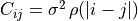$C_{ij} = \sigma^2 \, \rho(|i - j|)$ rather than its diagonal, correctly accounting for channel-to-channel noise correlation (e.g. from Hanning smoothing in the imaging pipeline). The ACF can be estimated directly from the cube with bettermoments.estimate_spectral_acf(), or enabled from the command line with the --acf flag. Only the uncertainty maps are affected — the moment values themselves are unchanged.

Moment Maps

Implementation of traditional moment-map methods. See the CASA documentation for more information.

bettermoments.methods.collapse_zeroth(velax, data, rms, acf=None)

Collapses the cube by integrating along the spectral axis. It will return the integrated intensity along the spectral axis, M0, and the associated uncertainty, dM0. Following Teague (2019) these are calculated by,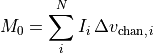

$M_0 = \sum_{i}^N I_i \, \Delta v_{{\rm chan},\,i}$

and

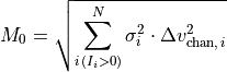
$M_0 = \sqrt{\sum_{i\,(I_i > 0)}^N \sigma_i^2 \cdot \Delta v_{{\rm chan},\,i}^2}$

where $\Delta v_i$ and $I_i$ are the chanenl width and flux density at the $i^{\rm th}$ channel, respectively and the sum goes over the whole axis.

If acf is provided, the uncertainty is propagated through the full spectral covariance matrix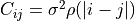 $C_{ij} = \sigma^2 \rho(|i - j|)$ rather than its diagonal, correctly accounting for noise correlation between channels (e.g.from Hanning smoothing). See bettermoments.estimate_spectral_acf().

Parameters:

velax (ndarray) – Velocity axis of the cube.
data (ndarray) – Flux densities or brightness temperature array. Assumes that the first axis is the velocity axis.
rms (float) – Noise per pixel in same units as data.
acf (Optional[ndarray]) – Normalised spectral ACF, e.g.from bettermoments.estimate_spectral_acf(). If None (default), channels are assumed independent.

Returns:

M0, the integrated intensity along provided axis and dM0, the uncertainty on M0 in the same units as M0.

Return type:

M0 (ndarray), dM0 (ndarray)

bettermoments.methods.collapse_first(velax, data, rms, acf=None)

Collapses the cube using the intensity weighted average velocity (or first moment map). For a symmetric line profile this will be the line center, however for highly non-symmetric line profiles, this will not give a meaningful result. Following Teague (2019), the line center is given by,

$M_1 = \frac{\sum_i^N I_i v_i}{\sum_i^N I_i}$

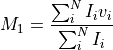
where $v_i$ and $I_i$ are the velocity and flux density at the $i^{\rm th}$ channel, respectively and the sum goes over the whole axis. In addition, the uncertainty is given by,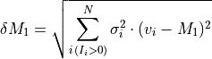

$\delta M_1 = \sqrt{\sum_{i\,(I_i > 0)}^N \sigma_i^2 \cdot (v_i - M_1)^2}$

where $\sigma_i$ is the rms noise.

If acf is provided, the uncertainty is propagated through the full spectral covariance rather than its diagonal — see collapse_zeroth().

Parameters:

velax (ndarray) – Velocity axis of the cube.
data (ndarray) – Flux densities or brightness temperature array. Assumes that the zeroth axis is the velocity axis.
rms (float) – Noise per pixel in same units as data.
acf (Optional[ndarray]) – Normalised spectral ACF. If None (default), channels are assumed independent.

Returns:

M1, the intensity weighted average velocity in units of velax and dM1, the uncertainty in the intensity weighted average velocity with same units as v0.

Return type:

M1 (ndarray), dM1 (ndarray)

bettermoments.methods.collapse_second(velax, data, rms, acf=None)

Collapses the cube using the intensity-weighted average velocity dispersion (or second moment). For a symmetric line profile this will be a measure of the line width. Following Teague (2019) this is calculated by,

$M_2 = \sqrt{\frac{\sum_i^N I_i (v_i - M_1)^2}{{\sum_i^N I_i}}}$

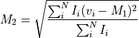
where $M_1$ is the first moment and $v_i$ and $I_i$ are the velocity and flux density at the $i^{\rm th}$ channel, respectively. The uncertainty is given by,

$\delta M_2 &= \frac{1}{2 M_2} \cdot \sqrt{\sum_{i\,(I_i > 0)}^N \sigma_i^2 \cdot \big[(v_i - M_1)^2 - M_2^2\big]^2}$

where $\sigma_i$ is the rms noise in the $i^{\rm th}$ channel.

If acf is provided, the uncertainty is propagated through the full spectral covariance rather than its diagonal — see collapse_zeroth().

Parameters:

velax (ndarray) – Velocity axis of the cube.
data (ndarray) – Flux densities or brightness temperature array. Assumes that the first axis is the velocity axis.
rms (float) – Noise per pixel in same units as data.
acf (Optional[ndarray]) – Normalised spectral ACF. If None (default), channels are assumed independent.

Returns:

M2 is the intensity weighted velocity dispersion with units of velax. dM2 is the uncertainty of M2 in the same units.

Return type:

M2 (ndarray), dM2 (ndarray)

bettermoments.methods.collapse_eighth(velax, data, rms)

Take the peak value along the provided axis. The uncertainty is the RMS noise of the image.

Parameters:

velax (ndarray) – Velocity axis of the cube. Not needed.
data (ndarray) – Flux densities or brightness temperature array. Assumes that the first axis is the velocity axis.
rms (float) – Noise per pixel in same units as data.

Returns:

The peak value, M8, and the associated uncertainty, dM8.

Return type:

M8 (ndarray), dM8 (ndarray)

bettermoments.methods.collapse_ninth(velax, data, rms)

Take the velocity of the peak intensity along the provided axis. The uncertainty is half the channel width.

Parameters:

velax (ndarray) – Velocity axis of the cube.
data (ndarray) – Flux densities or brightness temperature array. Assumes that the first axis is the velocity axis.
rms (float) – Noise per pixel in same units as data.

Returns:

The velocity value of the peak value, M9, and the associated uncertainty, dM9.

Return type:

M9 (ndarray), dM9 (ndarray)

bettermoments.methods.collapse_maximum(velax, data, rms)

A wrapper returning the result of both bettermoments.collapse_cube.collapse_eighth() and bettermoments.collapse_cube.collapse_ninth().

Parameters:

velax (ndarray) – Velocity axis of the cube.
data (ndarray) – Flux densities or brightness temperature array. Assumes that the first axis is the velocity axis.
rms (float) – Noise per pixel in same units as data.

Returns:

The peak value, M8, and the associated uncertainty, dM8. The velocity value of the peak value, M9, and the associated uncertainty, dM9.

Return type:

M8 (ndarray), dM8 (ndarray), M9 (ndarray), dM9 (ndarray)

Non-Traditional Methods

bettermoments.methods.collapse_quadratic(velax, data, rms, acf=None)

Collapse the cube using the quadratic method presented in Teague & Foreman-Mackey (2018). Will return the line center, v0, and the uncertainty on this, dv0, as well as the line peak, Fnu, and the uncertainty on that, dFnu. This provides the sub-channel precision of bettermoments.collapse_cube.collapse_first() with the robustness to noise from bettermoments.collapse_cube.collapse_ninth().

If acf is provided, the uncertainties are propagated through the 3x3 spectral covariance sub-block centred on the peak channel rather than the diagonal — see collapse_zeroth().

Parameters:

velax (ndarray) – Velocity axis of the cube.
data (ndarray) – Flux density or brightness temperature array. Assumes that the zeroth axis is the velocity axis.
rms (float) – Noise per pixel in same units as data.
acf (Optional[ndarray]) – Normalised spectral ACF. If None (default), channels are assumed independent.

Returns:

v0, the line center in the same units as velax with dv0 as the uncertainty on v0 in the same units as velax. Fnu is the line peak in the same units as the data with associated uncertainties, dFnu.

Return type:

v0 (ndarray), dv0 (ndarray), Fnu (ndarray), dFnu (ndarray)

bettermoments.methods.collapse_width(velax, data, rms, acf=None)

Returns an effective width, a rescaled ratio of the integrated intensity and the line peak. For a Gaussian line profile this would be the Doppler width as the total intensity is given by,

$M_0 = \sum_{i}^N I_i \, \Delta v_{{\rm chan},\,i}$

where $\Delta v_i$ and $I_i$ are the chanenl width and flux density at the $i^{\rm th}$ channel. If the line profile is Gaussian, then equally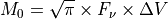

$M_0 = \sqrt{\pi} \times F_{\nu} \times \Delta V$

where $F_{\nu}$ is the peak value of the line and $\Delta V$ is the Doppler width of the line. As $M_0$ and $F_{\nu}$ are readily calculated using bettermoments.collapse_cube.collapse_zeroth() and bettermoments.collapse_cube.collapse_quadratic(), respectively, $\Delta V$ can calculated through $\Delta V = M_{0} \, / \, (\sqrt{\pi} \, F_{\nu})$ . This should be more robust against noise than second moment maps.

Parameters:

velax (ndarray) – Velocity axis of the cube.
data (ndarray) – Flux densities or brightness temperature array. Assumes that the first axis is the velocity axis.
rms (float) – Noise per pixel in same units as data.

Returns:

The effective velocity dispersion, dV and ddV, the associated uncertainty.

Return type:

dV (ndarray), ddV (ndarray)

bettermoments.methods.collapse_percentiles(velax, data, rms)

Collapse the cube by taking intensity-weighted percentiles. This can be thought of as an extension to the first and second moments which are intensity weighted averages and standard deviations. The advantage here is that by looking at the 16th and 84th percentile individually, we learn something about the skewness of the line (i.e., red-shifted side compared to the blue-shifted side) without assuming a line profile.

Parameters:

velax (ndarray) – Velocity axis of the cube.
data (ndarray) – Masked intensity or brightness temperature array. The first axis must be the velocity axis.
rms (float) – Noise per pixel in same units as data.

Returns:

Eight ndarray values: the intensity-weighted median: (wp50, dwp50), the blue- and red-shifted line widths (wpdVb, dwpdVb, wpdVr, dwpdVr), and the line center based on the center of the 16th and 84th percentile (wp1684, dwp1684).

Return type:

tuple

(Higher Order) Gaussian Fits

bettermoments.methods.collapse_gaussian(velax, data, rms, indices=None, ncpu=1, acf=None, **kwargs)

Collapse the cube by fitting a Gaussian line profile to each pixel. This function is a wrapper of collapse_analytical which provides more details about the arguments.

Parameters:

velax (ndarray) – Velocity axis of the cube.
data (ndarray) – Maksed intensity or brightness temperature array. The first axis must be the velocity axis.
rms (float) – Noise per pixel in same units as data.
indices (Optional[list]) – A list of pixels described by (y_idx, x_idx) tuples to fit. If none are provided, will fit all pixels.
ncpu (Optional[int]) – Number of worker processes to use. Defaults to 1 (serial). Set higher to parallelise across CPU cores.

Returns:

Six ndarray values: the Gaussian center (gv0,: dgv0), the Doppler line width (gdV, dgdV) and the line peak (gFnu, dgFnu).

Return type:

tuple

bettermoments.methods.collapse_gaussthick(velax, data, rms, indices=None, ncpu=1, acf=None, **kwargs)

Collapse the cube by fitting a Gaussian line profile with an optically thick core to each pixel. This function is a wrapper of collapse_analytical which provides more details about the arguments.

Parameters:

velax (ndarray) – Velocity axis of the cube.
data (ndarray) – Maksed intensity or brightness temperature array. The first axis must be the velocity axis.
rms (float) – Noise per pixel in same units as data.
indices (Optional[list]) – A list of pixels described by (y_idx, x_idx) tuples to fit. If none are provided, will fit all pixels.
ncpu (Optional[int]) – Number of worker processes to use. Defaults to 1 (serial). Set higher to parallelise across CPU cores.

Returns:

Eight ndarray values: the Gaussian center (gtv0,: dgtv0), the Doppler width (gtdV, dgtdV), the line peak (gtFnu, dgtFnu), and the effective optical depth (gttau, dgttau).

Return type:

tuple

bettermoments.methods.collapse_gausshermite(velax, data, rms, indices=None, ncpu=1, acf=None, **kwargs)

Collapse the cube by fitting a Gaussian line profile with an optically thick core to each pixel. This function is a wrapper of collapse_analytical which provides more details about the arguments.

Parameters:

velax (ndarray) – Velocity axis of the cube.
data (ndarray) – Maksed intensity or brightness temperature array. The first axis must be the velocity axis.
rms (float) – Noise per pixel in same units as data.
indices (Optional[list]) – A list of pixels described by (y_idx, x_idx) tuples to fit. If none are provided, will fit all pixels.
ncpu (Optional[int]) – Number of worker processes to use. Defaults to 1 (serial). Set higher to parallelise across CPU cores.

Returns:

Ten ndarray values: the Gaussian center (ghv0,: dghv0), the line peak (ghFnu, dghFnu), the Doppler width (ghdV, dghdV), the h3 asymmetry term (ghh3, dghh3) and the h4 kurtosis term (ghh4, dghh4).

Return type:

tuple

bettermoments.methods.collapse_doublegauss(velax, data, rms, indices=None, ncpu=1, acf=None, **kwargs)

Collapse the cube by fitting two Gaussian line profiles to each pixel. The first Gaussian component will be the peak of the two components. This function is a wrapper of collapse_analytical which provides more details about the arguments.

Parameters:

velax (ndarray) – Velocity axis of the cube.
data (ndarray) – Maksed intensity or brightness temperature array. The first axis must be the velocity axis.
rms (float) – Noise per pixel in same units as data.
indices (Optional[list]) – A list of pixels described by (y_idx, x_idx) tuples to fit. If none are provided, will fit all pixels.
ncpu (Optional[int]) – Number of worker processes to use. Defaults to 1 (serial). Set higher to parallelise across CPU cores.

Returns:

Twelve ndarray values: the primary Gaussian center: (ggv0, dggv0), line peak (ggFnu, dggFnu) and Doppler width (ggdV, dggdV), followed by the same for the secondary component (ggv0b, dggv0b, ggFnub, dggFnub, ggdVb, dggdVb).

Return type:

tuple

bettermoments.methods.collapse_analytical(velax, data, rms, model_function, indices=None, ncpu=1, acf=None, **kwargs)

Collapse the cube by fitting an analytical form to each pixel, including the option to use an MCMC sampler which has been found to be more forgiving when it comes to noisy data. Parallelism is handled at the per-pixel level so work is distributed evenly across workers.

For more information on kwargs, see the fit_spectrum documentation in mcmc_sampling.py.

Parameters:

velax (ndarray) – Velocity axis of the cube.
data (ndarray) – Masked intensity or brightness temperature array. The first axis must be the velocity axis.
rms (float) – Noise per pixel in same units as data.
model_function (str) – Name of the model function to fit to the data. Must be a function within profiles.py.
indices (Optional[list]) – A list of pixels described by (y_idx, x_idx) tuples to fit. If none are provided, will fit all pixels.
ncpu (Optional[int]) – Number of worker processes to use. Defaults to 1 (serial execution with no pool overhead). Set to a higher value to parallelise across CPU cores.

Returns:

An array containing all the fits. The first: axis contains the mean and standard deviation of each posterior distribution.

Return type:

results_array (ndarray)